Solving Bayesian Statistics Assignments with Confidence

Bayesian inference is a statistical method that incorporates prior knowledge with observed data to update our beliefs about uncertain parameters. Assignments in Bayesian inference typically involve deriving posterior distributions, selecting appropriate priors, and using computational methods such as Monte Carlo simulations. For students seeking statistics homework help, understanding these foundational concepts is crucial for tackling assignments effectively. This blog provides a structured approach to solving Bayesian inference assignments, particularly those involving normal models and multinomial distributions, closely aligned with real-world applications. Whether you are dealing with conjugate priors or computational simulations, a well-defined approach ensures clarity in problem-solving. Additionally, if you require help with Bayesian statistics homework, grasping these theoretical principles will aid in developing stronger analytical skills.

Understanding the Problem Statement

A well-defined Bayesian inference problem consists of observed data, a likelihood function, a prior distribution, a posterior distribution, and inference. The observed data represent the sample provided in the problem, while the likelihood function describes the probability distribution that explains the data generation process. The prior distribution encapsulates previous beliefs about the parameters before observing the data. Applying Bayes' theorem results in the posterior distribution, which integrates prior knowledge with the likelihood to refine parameter estimates. Finally, statistical inference involves analyzing the posterior distribution to derive meaningful conclusions. A well-defined Bayesian inference problem consists of:

• Observed Data: This is the sample data given in the problem.
• Likelihood Function: The probability distribution that describes how the data was generated.
• Prior Distribution: A mathematical representation of prior beliefs about parameters before observing the data.
• Posterior Distribution: The updated distribution obtained after incorporating the observed data.
• Inference and Interpretation: The final step involves drawing conclusions from the posterior distribution.

Selecting Priors and Their Justifications

Choosing an appropriate prior distribution is crucial in Bayesian inference. Conjugate priors simplify computation by ensuring that the posterior follows the same family as the prior. Non-informative priors, such as uniform or Jeffreys' priors, are used when prior knowledge is minimal. Empirical priors incorporate real-world data to inform parameter selection. For example, when modeling tennis serve times, a normal prior centered around historical mean serve times is appropriate. The justification for a prior depends on domain knowledge, mathematical convenience, and the problem's objectives, ensuring a well-balanced Bayesian analysis. Choosing an appropriate prior distribution is crucial in Bayesian inference. Priors can be:

• Conjugate Priors: These ensure that the posterior distribution follows the same family as the prior. For instance, in normal models, the conjugate prior for the mean and variance is the Normal-Inverse-Gamma distribution.
• Non-Informative Priors: These are used when no strong prior knowledge exists and are often chosen to be uniform or Jeffreys' priors.
• Empirical Priors: These are based on observed data and chosen to reflect real-world patterns.

For instance, when modeling serve times in tennis, a normal distribution with a mean based on previous tournament data serves as a reasonable prior.

Deriving Posterior Distributions

The posterior distribution, obtained via Bayes' theorem, combines the prior and likelihood to update parameter estimates. For normally distributed data with a Normal-Inverse-Gamma prior, the posterior follows the same family, simplifying analysis. In cases where analytical solutions are intractable, computational methods such as Markov Chain Monte Carlo (MCMC) can approximate the posterior. These methods iteratively sample from the distribution to generate a representative estimate. The posterior distribution provides insights into parameter uncertainties, enabling informed decision-making based on credible intervals and probability comparisons.

The posterior distribution is computed using Bayes' theorem:

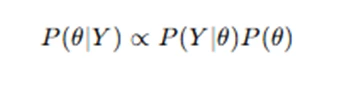
where P(Y∣θ) is the likelihood and P(θ) is the prior.

For normally distributed data with a Normal-Inverse-Gamma prior:

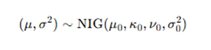
Updating this with observed data provides an analytically tractable posterior.

Computational Methods: Monte Carlo Simulations

Monte Carlo methods, such as Gibbs sampling and Metropolis-Hastings, approximate posterior distributions when analytical solutions are intractable. These methods involve drawing samples from probability distributions and using them to approximate expectations. The process begins with defining an appropriate prior, computing the likelihood function, and iteratively sampling from conditional distributions. Markov Chain Monte Carlo (MCMC) methods generate dependent samples that converge to the posterior distribution. By analyzing these posterior samples, credible intervals and parameter estimates can be obtained, providing insights into the statistical problem. Monte Carlo simulations are widely used in Bayesian inference, enabling the estimation of probabilities such as through repeated sampling and integration. When analytical solutions are intractable, Monte Carlo methods, such as Gibbs sampling and Metropolis-Hastings, approximate the posterior distribution. In practice:

• Define the Prior: Choose an appropriate prior distribution.
• Compute the Likelihood: Derive the probability of the data given the parameters.
• Draw Random Samples: Use Markov Chain Monte Carlo (MCMC) methods.
• Analyze Posterior Estimates: Compute credible intervals and probabilities of interest.

For example, estimating the probability that one tennis player has a longer serve time than another requires computing: P(μ1>μ2∣Y) using Monte Carlo integration.

Bayesian Modeling for Multinomial Data

When dealing with categorical data, a multinomial model is often used to describe the probability distribution of different outcomes. The likelihood function of a multinomially distributed variable is defined as 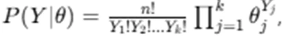where represents the probabilities associated with different categories. A common Bayesian prior for multinomial distributions is the Dirichlet distribution, which results in a conjugate posterior: 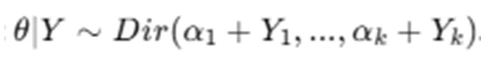The Dirichlet prior allows easy posterior updating by adjusting the hyperparameters based on observed counts. Bayesian modeling for multinomial data is useful in applications such as classification problems, voting behavior analysis, and language modeling, where prior beliefs about categorical probabilities are updated with observed data to make probabilistic predictions. When data consists of multiple categorical outcomes, a multinomial model is appropriate. The likelihood for a multinomially distributed variable is:

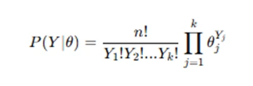
where θ represents the probabilities of different outcomes.

A common prior for multinomial distributions is the Dirichlet distribution, which leads to a convenient posterior:

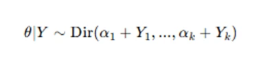
where α represents the prior pseudo-counts.

Making Statistical Comparisons

Statistical comparisons in Bayesian inference involve evaluating differences in parameters through posterior distributions. One common approach is to compute posterior probabilities such as to assess variability between two groups. Visualization techniques, including posterior density plots and scatterplots, help interpret parameter relationships. Bayesian credible intervals provide a probabilistic measure of uncertainty, offering insights into differences between groups. These methods are valuable in hypothesis testing and decision-making, where Bayesian inference allows probabilistic conclusions rather than binary accept/reject decisions. By leveraging posterior samples, Bayesian approaches provide a nuanced comparison framework that incorporates prior knowledge and observed data.,Assignments often require comparing distributions. Key steps include:

• Computing Posterior Probabilities: For example, finding 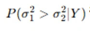gives insights into variance differences.
• Visualizing Posterior Samples: Scatterplots and histograms can reveal parameter relationships.
• Interpreting Findings: A high probability that μ1>μ2 suggests a significant difference between two groups.

Conclusion

Solving Bayesian inference assignments requires a structured approach that includes selecting appropriate priors, deriving posterior distributions, and using computational techniques like Monte Carlo simulations. Bayesian modeling provides a probabilistic framework for parameter estimation and comparison, allowing for more informed decision-making. Understanding the principles of Bayesian inference equips students with the skills to tackle complex statistical problems effectively. By integrating prior information with observed data, Bayesian methods offer a flexible and powerful approach to statistical analysis across various domains.