A Solution to Calculate Financial Statistics Assignment Using Excel and Finding the Internal Rate of Return

Assignment instructions

1. Pranjali Kashyap is a financial analyst at Mount Moreland Hospital in Baltimore, Maryland. She is using an Excel workbook to analyze the financial data for a proposed program called Neighborhood Nurse. The program involves nurses and nurse practitioners providing healthcare services to Baltimore neighborhoods from a van outfitted with medical equipment and supplies. She asks for your help in correcting errors and making financial calculations in the workbook.

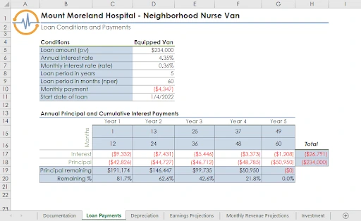
   Go to the Loan Payments worksheet. The hospital needs a loan to buy the medical van for the Neighborhood Nurse program. Before Pranjali can calculate the principal and interest payments on the loan, she asks you to correct the errors in the worksheet. Correct the first error as follows:

   1. In cell H17, use the Error Checking command to identify the error in the cell.
   2. Correct the error to total the values in the range C17:G17. In a later step, you will calculate the interest and principal in the range C17:G18 to remove the remaining errors.
2. Correct the #VALUE! errors in the worksheet as follows:
   1. Use Trace Precedents arrows to find the source of the #VALUE! error in cell C20.
   2. Correct the formula in cell C20, which should divide the remaining principal (cell C19) by the loan amount (cell D5) to find the percentage of the remaining principal.
   3. Fill the range D20:G20 with the formula in cell C20 to correct the remaining #VALUE! errors.
   4. Remove any remaining trace arrows.
3. Now Pranjali is ready to calculate the annual principal and interest payments for the medical van. Start by calculating the cumulative interest payments as follows:
   1. In cell C17, enter a formula using the CUMIPMT function to calculate the cumulative interest paid on the loan for Year 1 (payment 1 in cell C15 through payment 12 in cell C16). Use 0 as the type argument in your formula because payments are made at the end of the period.
   2. Use absolute references for the rate, nper, and pv arguments, which are listed in the range D5:D11.
   3. Use relative references for the start and end arguments.
   4. Fill the range D17:G17 with the formula in cell C17 to calculate the interest paid in Years 2–5 and the total interest.
4. Calculate the cumulative principal payments as follows:
   1. In cell C18, enter a formula using the CUMPRINC function to calculate the cumulative principal paid for Year 1 (payment 1 in cell C15 through payment 12 in cell C16). Use 0 as the type argument in your formula because payments are made at the end of the period.
   2. Use absolute references for the rate, nper, and pv arguments, which are listed in the range D5:D11.
   3. Use relative references for the start and end arguments.
   4. Fill the range D18:G18 with the formula in cell C18 to calculate the principal paid in Years 2–5 and the total principal.
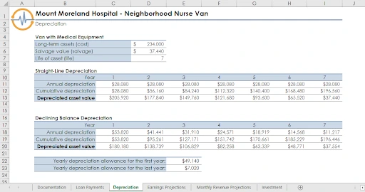
5. Go to the Depreciation worksheet. Pranjali needs to correct the errors on this worksheet before she can perform any depreciation calculations.

   Correct the errors as follows:

   1. Use Trace Dependents arrows to determine whether the #VALUE! error in cell D12 is causing the other errors in the worksheet.
   2. Use Trace Precedents arrows to find the source of the error in cell D12.
   3. Correct the error so that the formula in cell D12 calculates the cumulative straight-line depreciation of the medical van by adding the Cumulative depreciation value in Year 1 to the Annual depreciation value in Year 2.
6. Pranjali wants to compare straight-line depreciation amounts with declining balance depreciation amounts to determine which method is more favorable for the hospital's balance sheet. In the range D5:D7, she estimates that the Neighborhood Nurse program will have $234,000 in tangible assets at startup and that the useful life of these assets is seven years with a salvage value of $37,440.

   Start by calculating the straight-line depreciation amounts as follows:

   1. In cell C11, enter a formula using the SLN function to calculate the straight-line depreciation for the medical van during its first year of operation.
   2. Use absolute references for the cost, salvage, and life arguments in the SLN formula.
   3. Fill the range D11:I11 with the formula in cell C11 to calculate the annual and cumulative straight-line depreciation in Years 2–7.
7. Calculate the declining balance depreciation amounts for the medical van as follows:
   1. In cell C18, enter a formula using the DB function to calculate the declining balance depreciation for the medical van during its first year of operation.
   2. Use Year 1 (cell C17) as the current period.
   3. Use absolute references only for the cost, salvage, and life arguments in the DB formula.
   4. Fill the range D18:I18 with the formula in cell C18 to calculate the annual and cumulative declining balance depreciation in Years 2–7.
8. Pranjali also wants to determine the depreciation balance for the first year and the last year of the useful life of the medical van.

   Determine these amounts as follows:

   1. In cell E22, enter a formula using the SYD function to calculate the depreciation balance for the first year.
   2. Use Year 1 (cell C17) as the current period.
   3. In cell E23, enter a formula using the SYD function to calculate the depreciation balance for the last year.
   4. Use Year 7 (cell I17) as the current period.
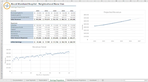
9. Go to the Earnings Projections worksheet. Pranjali has entered most of the income and expense data on the worksheet. She knows the income from municipal grants will be $25,000 in 2022, and estimates it will be $40,000 in 2026. She needs to calculate the income from municipal grants in the years 2023–2025. The grants should increase at a constant amount from year to year.

   Project the income from Municipal grants for 2023–2025 (cells D5:F5) using a Linear Trend interpolation.

10. Pranjali also needs to calculate the income from insurance reimbursements in the years 2023–2025. She knows the starting amount and has estimated the amount in 2026. She thinks this income will increase by a constant percentage.

    Project the income from Insurance reimbursements for 2023–2025 (cells D7:F7) using a Growth Trend interpolation.

11. Pranjali needs to calculate the payroll expenses in the years 2023–2026. She knows the payroll will be $140,000 in 2022 and will increase by at least five percent per year.

    Project the payroll expenses as follows:

    1. Project the expenses for Payroll for 2023-2026 (cells D13:G13) using a Growth Trend extrapolation.
    2. Use 1.05 (a 5 percent increase) as the step value.
12. The Projected Revenue line chart in the range H4:Q19 shows the revenue Pranjali estimates in the years 2022–2026. She wants to extend the projection into 2027.

    Modify the Projected Revenue line chart as follows to forecast the future trend:

    1. Add a Linear Trendline to the Projected Revenue line chart.
    2. Format the trendline to forecast 1 period forward.
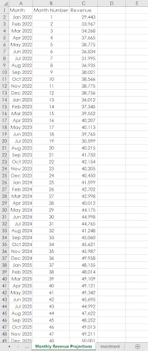
13. The Revenue Trend scatter chart in the range A21:G40 is based on monthly revenue estimates listed on the Monthly Revenue Projections worksheet. Pranjali wants to include a trendline for this chart that shows how revenues increase quickly at first and then level off in later months.

    Modify the Revenue Trend scatter chart as follows to include a logarithmic trendline:

    1. Add a Trendline to the Revenue Trend scatter chart.
    2. Format the trendline to use the Logarithmic option.
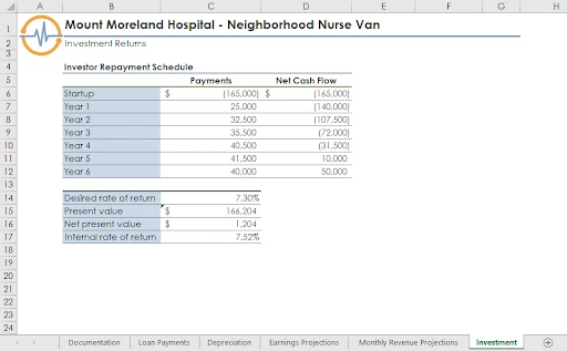
14. Go to the Investment worksheet. This worksheet should show the returns potential investors could realize if they invested $165,000 in the Neighborhood Nurse program. Pranjali figures a desirable rate of return would be 7.3 percent. She estimates the investment would pay different amounts each year (range C7:C12) and wants to calculate the present value of the investment.

    Calculate the present value of the investment as follows:

    1. In cell C15, enter a formula that uses the NPV function to calculate the present value of the investment in a medical van for the Neighborhood Nurse program.
    2. Use the desired rate of return value (cell C14) as the rate argument.
    3. Use the payments in Years 1–6 (range C7:C12) as the returns paid to investors. (Hint: If a Formula Omits Adjacent Cell error warning appears, ignore it.)
15. Pranjali also wants to calculate the internal rate of return on the investment. If it is 7 percent or higher, she is confident she can attract investors.

    Calculate the internal rate of return on the investment as follows:

    1. In cell C17, enter a formula that uses the IRR function to calculate the internal rate of return for investing in a medical van for the Neighborhood Nurse program.
    2. Use the payments for startups and Years 1–6 (range C6:C12) as the returns paid to investors.

Your workbook should look like the Final Figures on the following pages. Save your changes, close the workbook, and then exit Excel. Follow the directions on the SAM website to submit your completed project.

Assignment Solution

Final Figure 1: Loan Payments Worksheet

Final Figure 2: Depreciation Worksheet

Final Figure 3: Earnings Projections Worksheet

Final Figure 4: Monthly Revenue Projections Worksheet

Final Figure 5: Investment Worksheet